%sqlplot

New in version 0.5.2.

Note

%sqlplot requires matplotlib: pip install matplotlib and this example requires duckdb-engine: pip install duckdb-engine

%load_ext sql

%sql duckdb://

Connecting to 'duckdb://'

from pathlib import Path
from urllib.request import urlretrieve

if not Path("penguins.csv").is_file():
    urlretrieve(
        "https://raw.githubusercontent.com/mwaskom/seaborn-data/master/penguins.csv",
        "penguins.csv",
    )

%%sql
SELECT * FROM "penguins.csv" LIMIT 3

Running query in 'duckdb://'

species	island	bill_length_mm	bill_depth_mm	flipper_length_mm	body_mass_g	sex
Adelie	Torgersen	39.1	18.7	181	3750	MALE
Adelie	Torgersen	39.5	17.4	186	3800	FEMALE
Adelie	Torgersen	40.3	18.0	195	3250	FEMALE

Note

You can view the documentation and command line arguments by running %sqlplot?

%sqlplot boxplot

Note

To use %sqlplot boxplot, your SQL engine must support:

percentile_disc(...) WITHIN GROUP (ORDER BY ...)

Snowflake, Postgres, DuckDB, and others support this.

Shortcut: %sqlplot box

-t/--table Table to use (if using DuckDB: path to the file to query)

-s/--schema Schema to use (No need to pass if using a default schema)

-c/--column Column(s) to plot. You might pass one than one value (e.g., -c a b c)

-o/--orient Boxplot orientation (h for horizontal, v for vertical)

-w/--with Use a previously saved query as input data

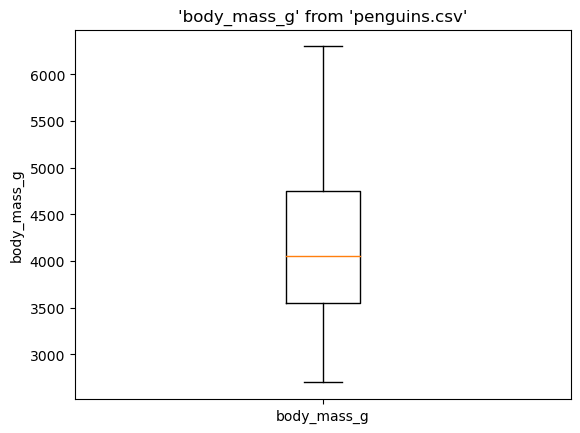
%sqlplot boxplot --table penguins.csv --column body_mass_g

<Axes: title={'center': "'body_mass_g' from 'penguins.csv'"}, ylabel='body_mass_g'>

Transform data before plotting

%%sql
SELECT island, COUNT(*)
FROM penguins.csv
GROUP BY island
ORDER BY COUNT(*) DESC

Running query in 'duckdb://'

island	count_star()
Biscoe	168
Dream	124
Torgersen	52

%%sql --save biscoe --no-execute
SELECT *
FROM penguins.csv
WHERE island = 'Biscoe'

Running query in 'duckdb://'

Skipping execution...

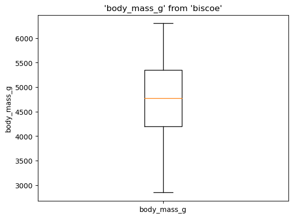
Since we saved biscoe from the cell above, we can pass it as an argument to --table since jupysql autogenerates the CTE.

%sqlplot boxplot --table biscoe --column body_mass_g

<Axes: title={'center': "'body_mass_g' from 'biscoe'"}, ylabel='body_mass_g'>

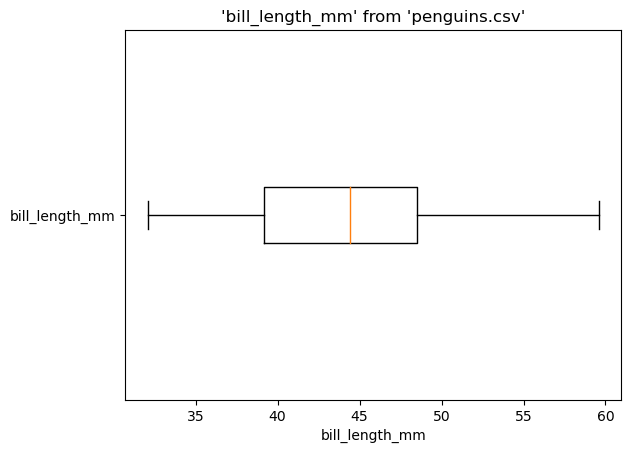
Horizontal boxplot

%sqlplot boxplot --table penguins.csv --column bill_length_mm --orient h

<Axes: title={'center': "'bill_length_mm' from 'penguins.csv'"}, xlabel='bill_length_mm'>

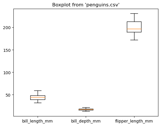
Multiple columns

%sqlplot boxplot --table penguins.csv --column bill_length_mm bill_depth_mm flipper_length_mm

<Axes: title={'center': "Boxplot from 'penguins.csv'"}>

%sqlplot histogram

Shortcut: %sqlplot hist

-t/--table Table to use (if using DuckDB: path to the file to query)

-s/--schema Schema to use (No need to pass if using a default schema)

-c/--column Column to plot

-b/--bins (default: 50) Number of bins

-B/--breaks Custom bin intervals

-W/--binwidth Width of each bin

-w/--with Use a previously saved query as input data

Note

When using -b/–bins, -B/–breaks, or -W/–binwidth, you can only specify one of them. If none of them is specified, the default value for -b/–bins will be used.

Histogram supports NULL values by skipping them. Now we can generate histograms without explicitly removing NULL entries.

New in version 0.7.9.

%sqlplot histogram --table penguins.csv --column body_mass_g 

<Axes: title={'center': "'body_mass_g' from 'penguins.csv'"}, xlabel='body_mass_g', ylabel='Count'>

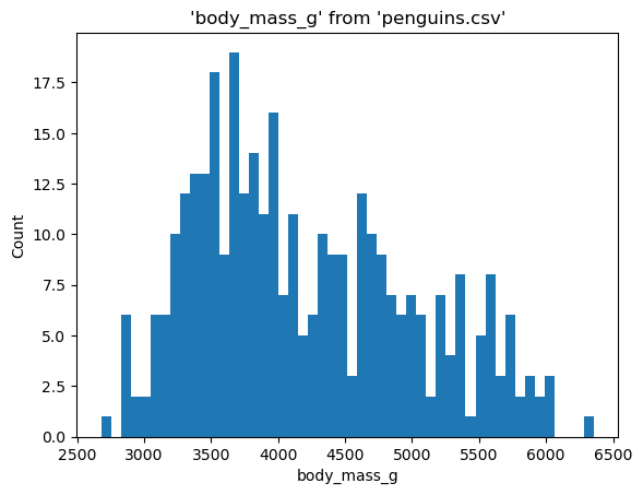
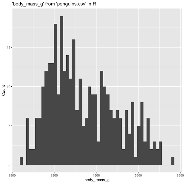
When plotting a histogram, it divides a range with the number of bins - 1 to calculate a bin size. Then, it applies round half down relative to the bin size and categorizes continuous values into bins to replicate right closed intervals from the ggplot histogram in R.

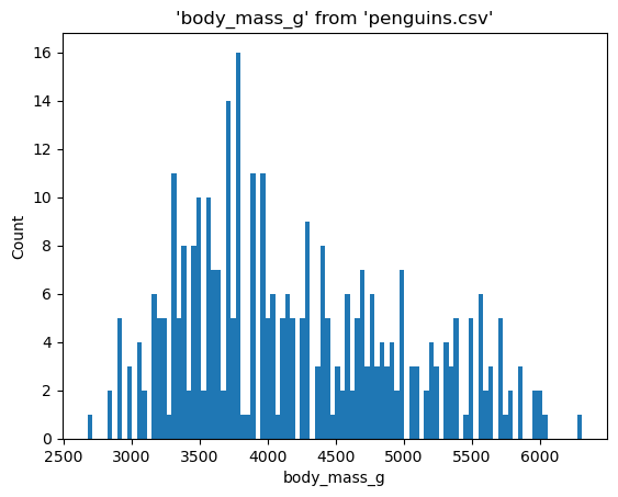
Specifying bins

Bins allow you to set the number of bins in a histogram, and it’s useful when you are interested in the overall distribution.

%sqlplot histogram --table penguins.csv --column body_mass_g  --bins 100

<Axes: title={'center': "'body_mass_g' from 'penguins.csv'"}, xlabel='body_mass_g', ylabel='Count'>

Specifying breaks

Breaks allow you to set custom intervals for a histogram. It is useful when you want to view distribution within a specific range. You can specify breaks by passing desired each end and break points separated by whitespace after -B/--breaks. Since those break points define a range of data points to plot, bar width, and number of bars in a histogram, make sure to pass more than 1 point that is strictly increasing and includes at least one data point.

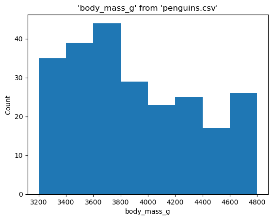
%sqlplot histogram --table penguins.csv --column body_mass_g --breaks 3200 3400 3600 3800 4000 4200 4400 4600 4800

<Axes: title={'center': "'body_mass_g' from 'penguins.csv'"}, xlabel='body_mass_g', ylabel='Count'>

Specifying binwidth

Binwidth allows you to set the width of bins in a histogram. It is useful when you directly aim to adjust the granularity of the histogram. To specify the binwidth, pass a desired width after -W/--binwidth. Since the binwidth determines details of distribution, make sure to pass a suitable positive numeric value based on your data.

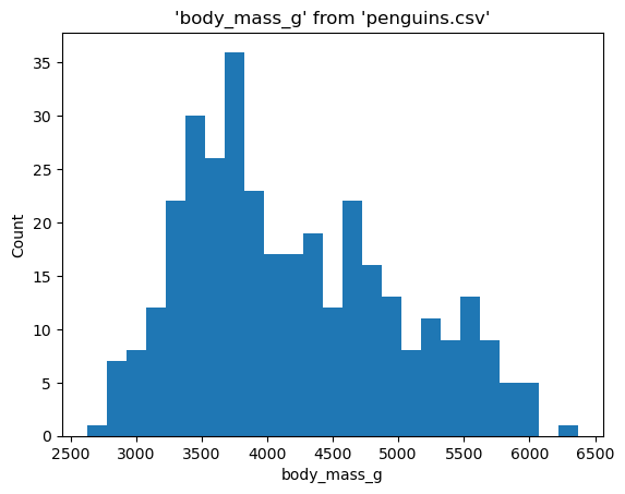
%sqlplot histogram --table penguins.csv --column body_mass_g --binwidth 150

<Axes: title={'center': "'body_mass_g' from 'penguins.csv'"}, xlabel='body_mass_g', ylabel='Count'>

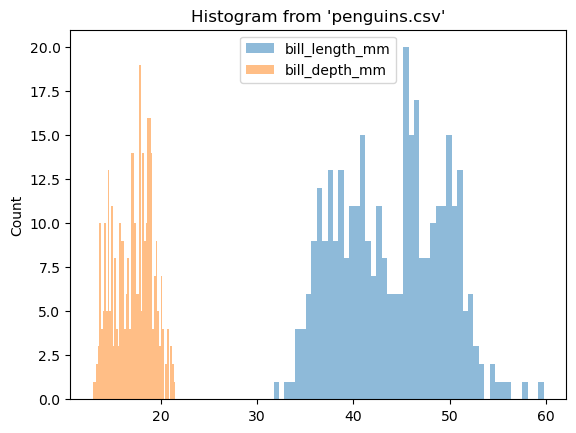
Multiple columns

%sqlplot histogram --table penguins.csv --column bill_length_mm bill_depth_mm 

<Axes: title={'center': "Histogram from 'penguins.csv'"}, ylabel='Count'>

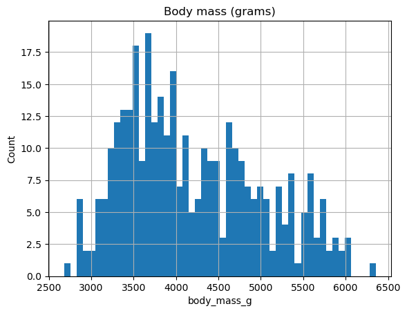
Customize plot

%sqlplot returns a matplotlib.Axes object.

ax = %sqlplot histogram --table penguins.csv --column body_mass_g
ax.set_title("Body mass (grams)")
_ = ax.grid()

%sqlplot bar

New in version 0.7.6.

Shortcut: %sqlplot bar

-t/--table Table to use (if using DuckDB: path to the file to query)

-s/--schema Schema to use (No need to pass if using a default schema)

-c/--column Column to plot.

-o/--orient Barplot orientation (h for horizontal, v for vertical)

-w/--with Use a previously saved query as input data

-S/--show-numbers Show numbers on top of the bar

Bar plot does not support NULL values, so we automatically remove them, when plotting.

%sqlplot bar --table penguins.csv --column species 

Removing NULLs, if there exists any from species

<Axes: title={'center': 'penguins.csv'}, xlabel='species', ylabel='Count'>

You can additionally pass two columns to bar plot i.e. x and height columns.

%%sql --save add_col --no-execute
SELECT species, count(species) as cnt
FROM penguins.csv
group by species

Running query in 'duckdb://'

Skipping execution...

%sqlplot bar --table add_col --column species cnt

Removing NULLs, if there exists any from species and cnt

<Axes: title={'center': 'add_col'}, xlabel='species', ylabel='cnt'>

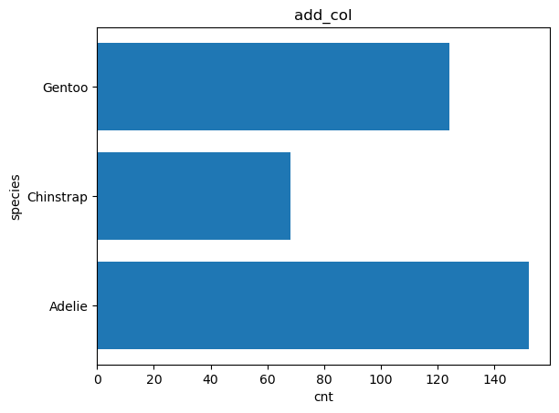
You can also pass the orientation using the orient argument.

%sqlplot bar --table add_col --column species cnt --orient h

Removing NULLs, if there exists any from species and cnt

<Axes: title={'center': 'add_col'}, xlabel='cnt', ylabel='species'>

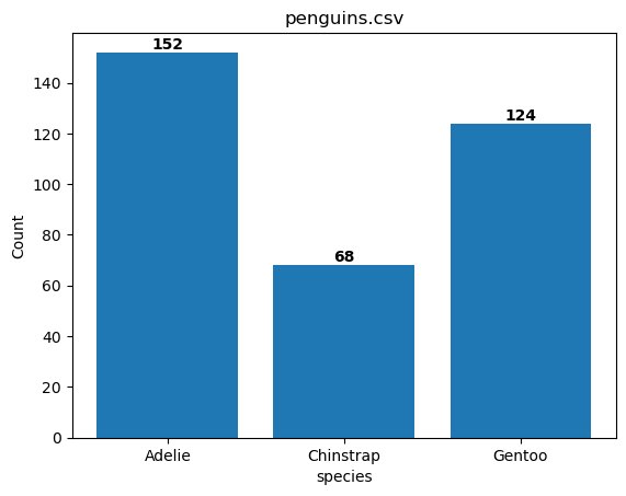
You can also show the number on top of the bar using the S/show-numbers argument.

%sqlplot bar --table penguins.csv --column species -S

Removing NULLs, if there exists any from species

<Axes: title={'center': 'penguins.csv'}, xlabel='species', ylabel='Count'>

%sqlplot pie

New in version 0.7.6.

Shortcut: %sqlplot pie

-t/--table Table to use (if using DuckDB: path to the file to query)

-s/--schema Schema to use (No need to pass if using a default schema)

-c/--column Column to plot

-w/--with Use a previously saved query as input data

-S/--show-numbers Show the percentage on top of the pie

Pie chart does not support NULL values, so we automatically remove them, when plotting the pie chart.

%sqlplot pie --table penguins.csv --column species

Removing NULLs, if there exists any from species

<Axes: title={'center': 'penguins.csv'}>

You can additionally pass two columns to bar plot i.e. labels and x columns.

%%sql --save add_col --no-execute
SELECT species, count(species) as cnt
FROM penguins.csv
group by species

Running query in 'duckdb://'

Skipping execution...

%sqlplot pie --table add_col --column species cnt

Removing NULLs, if there exists any from species and cnt

<Axes: title={'center': 'add_col'}>

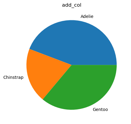
Here, species is the labels column and cnt is the x column.

You can also show the percentage on top of the pie using the S/show-numbers argument.

%sqlplot pie --table penguins.csv --column species -S

Removing NULLs, if there exists any from species

<Axes: title={'center': 'penguins.csv'}>

Parametrizing arguments

JupySQL supports variable expansion of arguments in the form of {{variable}}. This allows the user to specify arguments with placeholders that can be replaced by variables dynamically.

%%sql 
DROP TABLE IF EXISTS penguins;
CREATE SCHEMA IF NOT EXISTS s1;
CREATE TABLE s1.penguins (
    species VARCHAR(255),
    island VARCHAR(255),
    bill_length_mm DECIMAL(5, 2),
    bill_depth_mm DECIMAL(5, 2),
    flipper_length_mm DECIMAL(5, 2),
    body_mass_g INTEGER,
    sex VARCHAR(255)
);
COPY s1.penguins FROM 'penguins.csv' WITH (FORMAT CSV, HEADER TRUE);

Running query in 'duckdb://'

Count

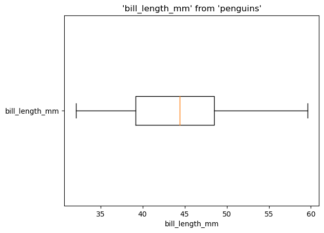
table = "penguins"
schema = "s1"
orient = "h"
column = "bill_length_mm"

%sqlplot boxplot --table {{table}} --schema {{schema}} --column {{column}} --orient {{orient}}

<Axes: title={'center': "'bill_length_mm' from 'penguins'"}, xlabel='bill_length_mm'>

Now let’s see another example using --with:

snippet = "gentoo"

%%sql --save {{snippet}}
SELECT * FROM {{schema}}.{{table}} 
WHERE species == 'Gentoo'

Running query in 'duckdb://'

species	island	bill_length_mm	bill_depth_mm	flipper_length_mm	body_mass_g	sex
Gentoo	Biscoe	46.10	13.20	211.00	4500	FEMALE
Gentoo	Biscoe	50.00	16.30	230.00	5700	MALE
Gentoo	Biscoe	48.70	14.10	210.00	4450	FEMALE
Gentoo	Biscoe	50.00	15.20	218.00	5700	MALE
Gentoo	Biscoe	47.60	14.50	215.00	5400	MALE
Gentoo	Biscoe	46.50	13.50	210.00	4550	FEMALE
Gentoo	Biscoe	45.40	14.60	211.00	4800	FEMALE
Gentoo	Biscoe	46.70	15.30	219.00	5200	MALE
Gentoo	Biscoe	43.30	13.40	209.00	4400	FEMALE
Gentoo	Biscoe	46.80	15.40	215.00	5150	MALE

Truncated to displaylimit of 10.

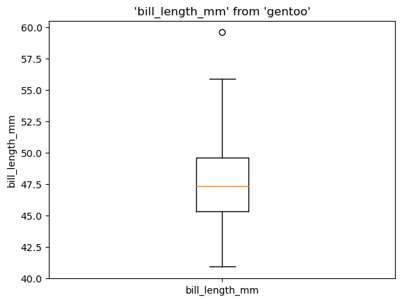
%sqlplot boxplot --table {{snippet}} --with {{snippet}} --column {{column}}

<Axes: title={'center': "'bill_length_mm' from 'gentoo'"}, ylabel='bill_length_mm'>