
Organizing Large Queries#
Required packages
pip install jupysql matplotlib
Changed in version 0.8.0.
Note
This is a beta feature, please join our community and let us know how we can improve it!
JupySQL allows you to break queries into multiple cells, simplifying the process of building large queries.
Simplify and modularize your workflow: JupySQL simplifies SQL queries and promotes code reusability by breaking down large queries into manageable chunks and enabling the creation of reusable query modules.
Seamless integration: JupySQL flawlessly combines the power of SQL with the flexibility of Jupyter Notebooks, offering a one-stop solution for all your data analysis needs.
Cross-platform compatibility: JupySQL supports popular databases like PostgreSQL, MySQL, SQLite, and more, ensuring you can work with any data source.
Example: record store data#
Goal:#
Using Jupyter notebooks, make a query against an SQLite database table named ‘Track’ with Rock and Metal song information. Find and show the artists with the most Rock and Metal songs. Show your results in a bar chart.
Data download and initialization#
Download the SQLite database file if it doesn’t exist
import urllib.request
from pathlib import Path

if not Path("my.db").is_file():
    url = "https://raw.githubusercontent.com/lerocha/chinook-database/master/ChinookDatabase/DataSources/Chinook_Sqlite.sqlite"  # noqa
    urllib.request.urlretrieve(url, "my.db")
Initialize the SQL extension and set autolimit=3 to only retrieve a few rows
%load_ext sql
%config SqlMagic.autolimit = 3
Query the track-level information from the Track table
%%sql sqlite:///my.db
SELECT * FROM Track
| TrackId | Name | AlbumId | MediaTypeId | GenreId | Composer | Milliseconds | Bytes | UnitPrice |
|---|---|---|---|---|---|---|---|---|
| 1 | For Those About To Rock (We Salute You) | 1 | 1 | 1 | Angus Young, Malcolm Young, Brian Johnson | 343719 | 11170334 | 0.99 |
| 2 | Balls to the Wall | 2 | 2 | 1 | None | 342562 | 5510424 | 0.99 |
| 3 | Fast As a Shark | 3 | 2 | 1 | F. Baltes, S. Kaufman, U. Dirkscneider & W. Hoffman | 230619 | 3990994 | 0.99 |
ResultSet : to convert to pandas, call .DataFrame() or to polars, call .PolarsDataFrame()Data wrangling#
Join the Track, Album, and Artist tables to get the artist name, and save the query as tracks_with_info
Note: --save stores the query, not the data
%%sql --save tracks_with_info
SELECT t.*, a.title AS album, ar.Name as artist
FROM Track t
JOIN Album a
USING (AlbumId)
JOIN Artist ar
USING (ArtistId)
| TrackId | Name | AlbumId | MediaTypeId | GenreId | Composer | Milliseconds | Bytes | UnitPrice | album | artist |
|---|---|---|---|---|---|---|---|---|---|---|
| 1 | For Those About To Rock (We Salute You) | 1 | 1 | 1 | Angus Young, Malcolm Young, Brian Johnson | 343719 | 11170334 | 0.99 | For Those About To Rock We Salute You | AC/DC |
| 2 | Balls to the Wall | 2 | 2 | 1 | None | 342562 | 5510424 | 0.99 | Balls to the Wall | Accept |
| 3 | Fast As a Shark | 3 | 2 | 1 | F. Baltes, S. Kaufman, U. Dirkscneider & W. Hoffman | 230619 | 3990994 | 0.99 | Restless and Wild | Accept |
ResultSet : to convert to pandas, call .DataFrame() or to polars, call .PolarsDataFrame()Filter genres we are interested in (Rock and Metal) and save the query as genres_fav
%%sql --save genres_fav
SELECT * FROM Genre
WHERE Name
LIKE '%rock%'
OR Name LIKE '%metal%'
| GenreId | Name |
|---|---|
| 1 | Rock |
| 3 | Metal |
| 5 | Rock And Roll |
ResultSet : to convert to pandas, call .DataFrame() or to polars, call .PolarsDataFrame()Join the filtered genres and tracks, so we only get Rock and Metal tracks, and save the query as track_fav
We automatically extract the tables from the query and infer the dependencies from all the saved snippets.
%%sql --save track_fav
SELECT t.*
FROM tracks_with_info t
JOIN genres_fav
ON t.GenreId = genres_fav.GenreId
| TrackId | Name | AlbumId | MediaTypeId | GenreId | Composer | Milliseconds | Bytes | UnitPrice | album | artist |
|---|---|---|---|---|---|---|---|---|---|---|
| 1 | For Those About To Rock (We Salute You) | 1 | 1 | 1 | Angus Young, Malcolm Young, Brian Johnson | 343719 | 11170334 | 0.99 | For Those About To Rock We Salute You | AC/DC |
| 2 | Balls to the Wall | 2 | 2 | 1 | None | 342562 | 5510424 | 0.99 | Balls to the Wall | Accept |
| 3 | Fast As a Shark | 3 | 2 | 1 | F. Baltes, S. Kaufman, U. Dirkscneider & W. Hoffman | 230619 | 3990994 | 0.99 | Restless and Wild | Accept |
ResultSet : to convert to pandas, call .DataFrame() or to polars, call .PolarsDataFrame()Now let’s find artists with the most Rock and Metal tracks, and save the query as top_artist
%%sql --save top_artist
SELECT artist, COUNT(*) FROM track_fav
GROUP BY artist
ORDER BY COUNT(*) DESC
| artist | COUNT(*) |
|---|---|
| Iron Maiden | 204 |
| Led Zeppelin | 114 |
| U2 | 112 |
ResultSet : to convert to pandas, call .DataFrame() or to polars, call .PolarsDataFrame()Note
A saved snippet will override an existing table with the same name during query formation. If you wish to delete a snippet please refer to sqlcmd snippets API.
Data visualization#
Once we have the desired results from the query top_artist, we can generate a visualization using the bar method
top_artist = %sql SELECT * FROM top_artist
top_artist.bar()
<Axes: xlabel='artist', ylabel='COUNT(*)'>
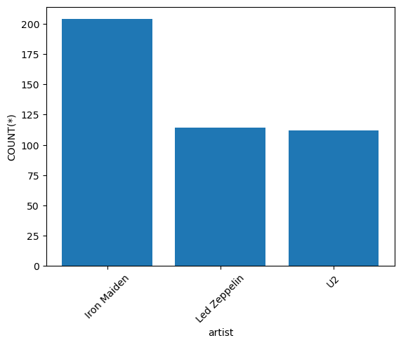
It looks like Iron Maiden had the highest number of rock and metal songs in the table.
We can render the full query with the %sqlcmd snippets {name} magic:
final = %sqlcmd snippets top_artist
print(final)
WITH `tracks_with_info` AS (
SELECT t.*, a.title AS album, ar.Name as artist
FROM Track t
JOIN Album a
USING (AlbumId)
JOIN Artist ar
USING (ArtistId)), `genres_fav` AS (
SELECT * FROM Genre
WHERE Name
LIKE '%rock%'
OR Name LIKE '%metal%' ), `track_fav` AS (
SELECT t.*
FROM tracks_with_info t
JOIN genres_fav
ON t.GenreId = genres_fav.GenreId)
SELECT artist, COUNT(*) FROM track_fav
GROUP BY artist
ORDER BY COUNT(*) DESC
We can verify the retrieved query returns the same result:
%%sql
{{final}}
| artist | COUNT(*) |
|---|---|
| Iron Maiden | 204 |
| Led Zeppelin | 114 |
| U2 | 112 |
ResultSet : to convert to pandas, call .DataFrame() or to polars, call .PolarsDataFrame()--with argument#
JupySQL also allows you to specify the snippet name explicitly by passing the --with argument. This is particularly useful when our parsing logic is unable to determine the table name due to dialect variations. For example, consider the below example:
%sql duckdb://
%%sql --save first_cte --no-execute
SELECT 1 AS column1, 2 AS column2
%%sql --save second_cte --no-execute
SELECT
  sum(column1),
  sum(column2) FILTER (column2 = 2)
FROM first_cte
%%sql
SELECT * FROM second_cte
UsageError: If using snippets, you may pass the --with argument explicitly.
For more details please refer : https://jupysql.ploomber.io/en/latest/compose.html#with-argument


Original error message from DB driver:
(duckdb.CatalogException) Catalog Error: Table with name first_cte does not exist!
Did you mean "pg_type"?
[SQL: WITH second_cte AS (
SELECT
  sum(column1),
  sum(column2) FILTER (column2 = 2)
FROM first_cte)
SELECT * FROM second_cte]
(Background on this error at: https://sqlalche.me/e/14/f405)
Note that the query fails because the clause FILTER (column2 = 2) makes it difficult for the parser to extract the table name. While this syntax works on some dialects like DuckDB, the more common usage is to specify WHERE clause as well, like FILTER (WHERE column2 = 2).
Now let’s run the same query by specifying --with argument.
%%sql --with first_cte --save second_cte --no-execute
SELECT
  sum(column1),
  sum(column2) FILTER (column2 = 2)
FROM first_cte
%%sql
SELECT * FROM second_cte
| sum(column1) | sum(column2) FILTER (WHERE (column2 = 2)) |
|---|---|
| 1 | 2 |
ResultSet : to convert to pandas, call .DataFrame() or to polars, call .PolarsDataFrame()Summary#
In the given example, we demonstrated JupySQL’s usage as a tool for managing large SQL queries in Jupyter Notebooks. It effectively broke down a complex query into smaller, organized parts, simplifying the process of analyzing a record store’s sales database. By using JupySQL, users can easily maintain and reuse their queries, enhancing the overall data analysis experience.