Redshift

Important

sqlalchemy-redshift requires SQLAlchemy 1.x (as of version 0.8.14)

This tutorial will show you how to use JupySQL with Redshift, a data warehouse service provided by AWS.

Pre-requisites

First, let’s install the required packages.

%pip install jupysql sqlalchemy-redshift redshift-connector 'sqlalchemy<2' --quiet

Note: you may need to restart the kernel to use updated packages.

Load JupySQL:

%load_ext sql

Found pyproject.toml from '/Users/eduardo/dev/jupysql'

Connect to Redshift

Here, we create a connection and pass it to JupySQL:

from os import environ
from sqlalchemy import create_engine
from sqlalchemy.engine import URL

user = environ["REDSHIFT_USERNAME"]
password = environ["REDSHIFT_PASSWORD"]
host = environ["REDSHIFT_HOST"]

url = URL.create(
    drivername="redshift+redshift_connector",
    username=user,
    password=password,
    host=host,
    port=5439,
    database="dev",
)

engine = create_engine(url)

%sql engine --alias redshift-sqlalchemy

Load data

We’ll load some sample data. First, we create the table:

%%sql
DROP TABLE taxi;

CREATE TABLE taxi  (
    VendorID                BIGINT,
    tpep_pickup_datetime    TIMESTAMP,
    tpep_dropoff_datetime   TIMESTAMP,
    passenger_count         DOUBLE PRECISION,
    trip_distance           DOUBLE PRECISION,
    RatecodeID              DOUBLE PRECISION,
    store_and_fwd_flag      VARCHAR(1),
    PULocationID            BIGINT,
    DOLocationID            BIGINT,
    payment_type            BIGINT,
    fare_amount             DOUBLE PRECISION,
    extra                   DOUBLE PRECISION,
    mta_tax                 DOUBLE PRECISION,
    tip_amount              DOUBLE PRECISION,
    tolls_amount            DOUBLE PRECISION,
    improvement_surcharge   DOUBLE PRECISION,
    total_amount            DOUBLE PRECISION,
    congestion_surcharge    DOUBLE PRECISION,
    airport_fee             DOUBLE PRECISION
);

Running query in 'redshift-sqlalchemy'

ResultSet : to convert to pandas, call .DataFrame() or to polars, call .PolarsDataFrame()

Now, we use COPY to copy a .parquet file stored in an S3 bucket:

Instructions to upload to S3

If you don’t have existing data and a role configured, here are the commands to do it:

Create bucket:

aws s3api create-bucket --bucket {bucket-name} --region {aws-region}

Download some sample data from here.

Upload to the S3 bucket:

aws s3 cp path/to/data.parquet s3://{bucket-name}/data.parquet

Create a role that allows Redshift to have S3 read access:

aws iam create-role --role-name {role-name} \
    --assume-role-policy-document '{"Version":"2012-10-17","Statement":[{"Effect":"Allow","Principal":{"Service":"redshift.amazonaws.com"},"Action":"sts:AssumeRole"}]}'
    
aws iam attach-role-policy --role-name {role-name} --policy-arn arn:aws:iam::aws:policy/AmazonS3ReadOnlyAccess

Then, go to the Redshift console and attach the role you created to your Redshift cluster.

%%sql
COPY taxi
FROM 's3:///some-bucket/yellow_tripdata_2023-01.parquet'
IAM_ROLE 'arn:aws:iam::XYZ:role/some-role'
FORMAT AS PARQUET;

Query

%%sql
SELECT * FROM taxi LIMIT 3

Running query in 'redshift-sqlalchemy'

vendorid	tpep_pickup_datetime	tpep_dropoff_datetime	passenger_count	trip_distance	ratecodeid	store_and_fwd_flag	pulocationid	dolocationid	payment_type	fare_amount	extra	mta_tax	tip_amount	tolls_amount	improvement_surcharge	total_amount	congestion_surcharge	airport_fee
2	2023-01-01 01:11:31	2023-01-01 01:21:50	1.0	4.59	1.0	N	132	139	2	-20.5	-1.0	-0.5	0.0	0.0	-1.0	-24.25	0.0	-1.25
2	2023-01-01 01:11:31	2023-01-01 01:21:50	1.0	4.59	1.0	N	132	139	2	20.5	1.0	0.5	0.0	0.0	1.0	24.25	0.0	1.25
2	2023-01-01 01:06:46	2023-01-01 01:42:58	5.0	6.8	1.0	N	68	179	1	36.6	1.0	0.5	8.32	0.0	1.0	49.92	2.5	0.0

ResultSet : to convert to pandas, call .DataFrame() or to polars, call .PolarsDataFrame()

Pandas/Polars integration

Tip

Learn more about the pandas and polars integrations.

You can convert results to pandas and polars data frames

%%sql results <<
SELECT tpep_pickup_datetime, tpep_dropoff_datetime FROM taxi LIMIT 100

Running query in 'redshift-sqlalchemy'

results.DataFrame().head()

	tpep_pickup_datetime	tpep_dropoff_datetime
0	2023-01-01 01:30:53	2023-01-01 02:03:29
1	2023-01-01 01:28:54	2023-01-01 01:53:11
2	2023-01-01 01:54:52	2023-01-01 02:00:54
3	2023-01-01 01:25:54	2023-01-01 01:35:49
4	2023-01-01 01:54:10	2023-01-01 02:11:43

results.PolarsDataFrame().head()

shape: (5, 2)

tpep_pickup_datetime	tpep_dropoff_datetime
datetime[μs]	datetime[μs]
2023-01-01 01:30:53	2023-01-01 02:03:29
2023-01-01 01:28:54	2023-01-01 01:53:11
2023-01-01 01:54:52	2023-01-01 02:00:54
2023-01-01 01:25:54	2023-01-01 01:35:49
2023-01-01 01:54:10	2023-01-01 02:11:43

List tables

%sqlcmd tables

Name
taxi

List columns

%sqlcmd columns --table taxi

name	type	nullable	default	autoincrement	comment	info
vendorid	BIGINT	True	None	False	None	{'encode': 'az64'}
tpep_pickup_datetime	TIMESTAMP	True	None	False	None	{'encode': 'az64'}
tpep_dropoff_datetime	TIMESTAMP	True	None	False	None	{'encode': 'az64'}
passenger_count	DOUBLE_PRECISION	True	None	False	None	{}
trip_distance	DOUBLE_PRECISION	True	None	False	None	{}
ratecodeid	DOUBLE_PRECISION	True	None	False	None	{}
store_and_fwd_flag	VARCHAR(1)	True	None	False	None	{'encode': 'lzo'}
pulocationid	BIGINT	True	None	False	None	{'encode': 'az64'}
dolocationid	BIGINT	True	None	False	None	{'encode': 'az64'}
payment_type	BIGINT	True	None	False	None	{'encode': 'az64'}
fare_amount	DOUBLE_PRECISION	True	None	False	None	{}
extra	DOUBLE_PRECISION	True	None	False	None	{}
mta_tax	DOUBLE_PRECISION	True	None	False	None	{}
tip_amount	DOUBLE_PRECISION	True	None	False	None	{}
tolls_amount	DOUBLE_PRECISION	True	None	False	None	{}
improvement_surcharge	DOUBLE_PRECISION	True	None	False	None	{}
total_amount	DOUBLE_PRECISION	True	None	False	None	{}
congestion_surcharge	DOUBLE_PRECISION	True	None	False	None	{}
airport_fee	DOUBLE_PRECISION	True	None	False	None	{}

Profile a dataset

%sqlcmd profile --table taxi

Following statistics are not available in redshift_connector: STD, 25%, 50%, 75%

	vendorid	tpep_pickup_datetime	tpep_dropoff_datetime	passenger_count	trip_distance	ratecodeid	store_and_fwd_flag	pulocationid	dolocationid	payment_type	fare_amount	extra	mta_tax	tip_amount	tolls_amount	improvement_surcharge	total_amount	congestion_surcharge	airport_fee
count	3066766	3066766	3066766	2995023	3066766	2995023	2995023	3066766	3066766	3066766	3066766	3066766	3066766	3066766	3066766	3066766	3066766	2995023	2995023
unique	2	1610975	1611319	10	4387	7	2	257	261	5	6873	68	10	4036	776	5	15871	3	3
mean	1.0000	nan	nan	1.3625	3.8473	1.4974	nan	166.0000	164.0000	1.0000	18.3671	1.5378	0.4883	3.3679	0.5185	0.9821	27.0204	2.2742	0.1074
min	1	nan	nan	0.0	0.0	1.0	nan	1	1	0	-900.0	-7.5	-0.5	-96.22	-65.0	-1.0	-751.0	-2.5	-1.25
max	2	nan	nan	9.0	258928.15	99.0	nan	265	265	4	1160.1	12.5	53.16	380.8	196.99	1.0	1169.4	2.5	1.25

Plotting

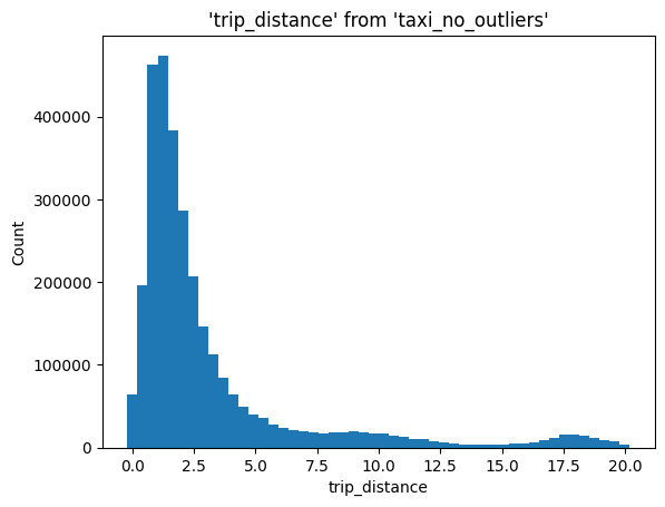
Let’s create a histogram for the trip_distance. Since there are outliers, we’ll use the 99th percentile as a cutoff value.

%%sql
SELECT 
    APPROXIMATE PERCENTILE_DISC(0.99) WITHIN GROUP (ORDER BY trip_distance)
FROM 
    taxi;

Running query in 'redshift-sqlalchemy'

percentile_disc
20.0

ResultSet : to convert to pandas, call .DataFrame() or to polars, call .PolarsDataFrame()

Let’s create a new snippet by filtering out the outliers using --save:

%%sql --save taxi_no_outliers --no-execute
select * from taxi  where trip_distance < 20

Running query in 'redshift-sqlalchemy'

Skipping execution...

Histogram

%sqlplot histogram --table taxi_no_outliers --column trip_distance

Plotting using saved snippet : taxi_no_outliers

<Axes: title={'center': "'trip_distance' from 'taxi_no_outliers'"}, xlabel='trip_distance', ylabel='Count'>

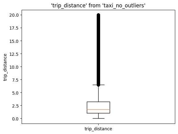
Boxplot

%sqlplot boxplot --table taxi_no_outliers --column trip_distance

Plotting using saved snippet : taxi_no_outliers

<Axes: title={'center': "'trip_distance' from 'taxi_no_outliers'"}, ylabel='trip_distance'>

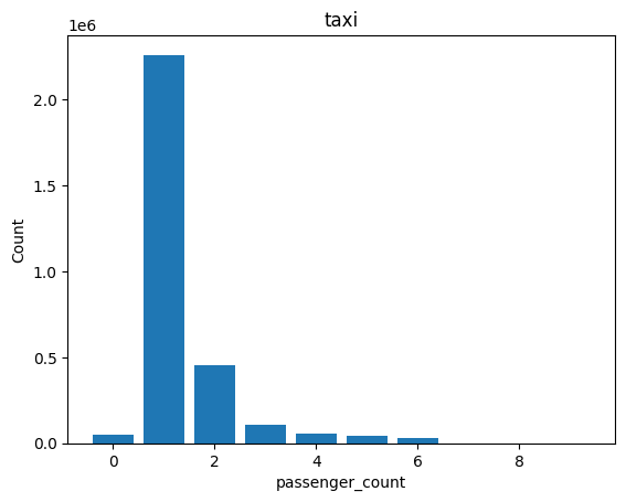
Bar

%sqlplot bar --table taxi --column passenger_count

Removing NULLs, if there exists any from passenger_count

<Axes: title={'center': 'taxi'}, xlabel='passenger_count', ylabel='Count'>

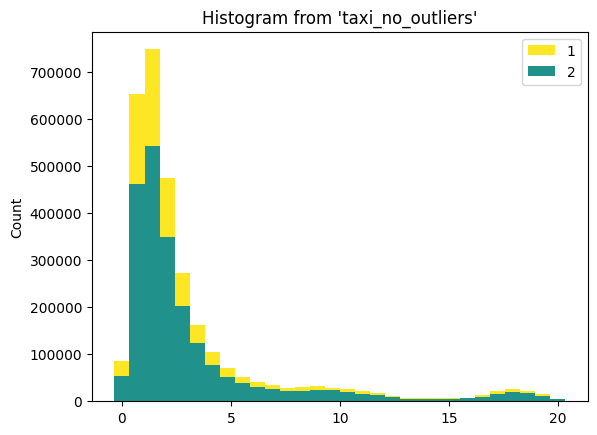
Plotting using the ggplot API

You can also use the ggplot API to create visualizations:

from sql.ggplot import ggplot, aes, geom_histogram

(
    ggplot("taxi_no_outliers", aes(x="trip_distance"), with_="taxi_no_outliers")
    + geom_histogram(bins=30, fill="vendorid")
)

<sql.ggplot.ggplot.ggplot at 0x15e0bae30>

Using a native connection

Using a native connection is also supported.

%pip install redshift-connector --quiet

Note: you may need to restart the kernel to use updated packages.

import redshift_connector

conn = redshift_connector.connect(
    host=host,
    database="dev",
    port=5439,
    user=user,
    password=password,
    timeout=60,
)

%sql conn --alias redshift-native